
What are the main characteristics which have the most impact on the car price?
import pandas as pd
import numpy as np
1) import data from the external source
path='https://cf-courses-data.s3.us.cloud-object-storage.appdomain.cloud/IBMDeveloperSkillsNetwork-DA0101EN-SkillsNetwork/labs/Data%20files/automobileEDA.csv'
df = pd.read_csv(path)
df.head()
2) install seaborn and matplotlib for visualization
%%capture
! pip install seaborn

import matplotlib.pyplot as plt
import seaborn as sns
%matplotlib inline
3) check the data types of each column
print(df.dtypes)4) <Continuous Numerical Variables>
- by using "regplot(plots scatterplot + the fitted regression line)", we can understand the linear relationship between an individual variable(continuous numerical - int64 or float64) and the price
* Positive Linear Relationship
# Engine size as potential predictor variable of price
sns.regplot(x="engine-size", y="price", data=df)
plt.ylim(0,)
->As the engine-size goes up, the price goes up: this indicates a positive direct correlation between these two variables. Engine size seems like a pretty good predictor of price since the regression line is almost a perfect diagonal line. We can examine the correlation(using corr()) between 'engine-size' and 'price' and see it's approximately 0.87
* Negative Linear Relationship
sns.regplot(x="highway-mpg", y="price", data=df)
* Weak Linear Relationship
sns.regplot(x="peak-rpm", y="price", data=df)
-> Peak rpm does not seem like a good predictor of the price at all since the regression line is close to horizontal. Also, the data points are very scattered and far from the fitted line, showing lots of variability. Therefore it's it is not a reliable variable.
5) Using Pearson Correlation
** Pearson Correlation
- The Pearson Correlation measures the linear dependence between two variables X and Y.
- The resulting coefficient is a value between -1 and 1 inclusive, where:
- 1: Total positive linear correlation.
- 0: No linear correlation, the two variables most likely do not affect each other.
- -1: Total negative linear correlation.
** P-value
- p-value is << 0.001: we say there is strong evidence that the correlation is significant.
- the p-value is << 0.05: there is moderate evidence that the correlation is significant.
- the p-value is << 0.1: there is weak evidence that the correlation is significant.
- the p-value is >> 0.1: there is no evidence that the correlation is significant.
* What is this P-value? The P-value is the probability value that the correlation between these two variables is statistically significant. Normally, we choose a significance level of 0.05, which means that we are 95% confident that the correlation between the variables is significant.
from scipy import stats

pearson_coef, p_value = stats.pearsonr(df['curb-weight'], df['price'])
print( "The Pearson Correlation Coefficient is", pearson_coef, " with a P-value of P = ", p_value)
- The Pearson Correlation Coefficient is 0.8344145257702846 with a P-value of P = 2.1895772388936914e-53
-> Since the p-value is << 0.001, the correlation between engine-size and price is statistically significant, and the linear relationship is very strong (~0.872)
- we can do this in every continuous numerical variables
6) <Categorical Variables> (using visualization - boxplot)
- These are variables that describe a 'characteristic' of a data unit, and are selected from a small group of categories. The categorical variables can have the type "object" or "int64". A good way to visualize categorical variables is by using boxplots.
sns.boxplot(x="body-style", y="price", data=df)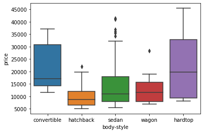
-> We see that the distributions of price between the different body-style categories have a significant overlap, and so body-style would not be a good predictor of price
sns.boxplot(x="engine-location", y="price", data=df)
-> the distribution of price between these two engine-location categories, front and rear, are distinct enough to take engine-location as a potential good predictor of price
- but when we use value_counts(), results are skewed
- we only have three cars with a rear engine and 198 with an engine in the front
# engine-location as variable
engine_loc_counts = df['engine-location'].value_counts().to_frame()
engine_loc_counts.rename(columns={'engine-location': 'value_counts'}, inplace=True)
engine_loc_counts.index.name = 'engine-location'
engine_loc_counts.head(10)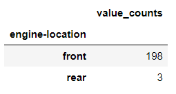
- Thus, we are not able to draw any conclusions about the engine location
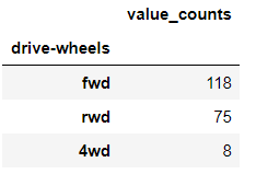
- when we use value_counts on "drive-wheels" variable, we can differentiate enough between "drive-wheels" types
7) ANOVA (Analysis of Variance) - categorical variable
= a statistical method used to test whether there are significant differences between the means of two or more groups
* ANOVA returns two parameters:
- F-test score: ANOVA assumes the means of all groups are the same, calculates how much the actual means deviate from the assumption, and reports it as the F-test score. A larger score means there is a larger difference between the means.
- P-value: P-value tells how statistically significant is our calculated score value.
- Since ANOVA analyzes the difference between different groups of the same variable, the groupby function will come in handy. Because the ANOVA algorithm averages the data automatically, we do not need to take the average before hand
ex)
df_gptest = df[['drive-wheels','body-style','price']]
grouped_test2=df_gptest[['drive-wheels', 'price']].groupby(['drive-wheels'])
grouped_test2.head(2)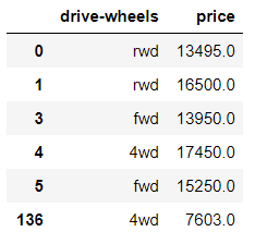
grouped_test2.get_group('4wd')['price']
# ANOVA
f_val, p_val = stats.f_oneway(grouped_test2.get_group('fwd')['price'], grouped_test2.get_group('rwd')['price'], grouped_test2.get_group('4wd')['price'])

print( "ANOVA results: F=", f_val, ", P =", p_val)
-> ANOVA results: F= 67.95406500780399 , P = 3.3945443577151245e-23
- This is a great result, with a large F test score showing a strong correlation and a P value of almost 0 implying almost certain statistical significance
- but when inspected separately from each of the groups with the other group, some groups show a small F
<<Conclusion>>
based on 4) & 5)
Continuous numerical variables:
- Length
- Width
- Curb-weight
- Engine-size
- Horsepower
- City-mpg
- Highway-mpg
- Wheel-base
- Bore
based on 6) & 7)
Categorical variables:
- Drive-wheels
댓글